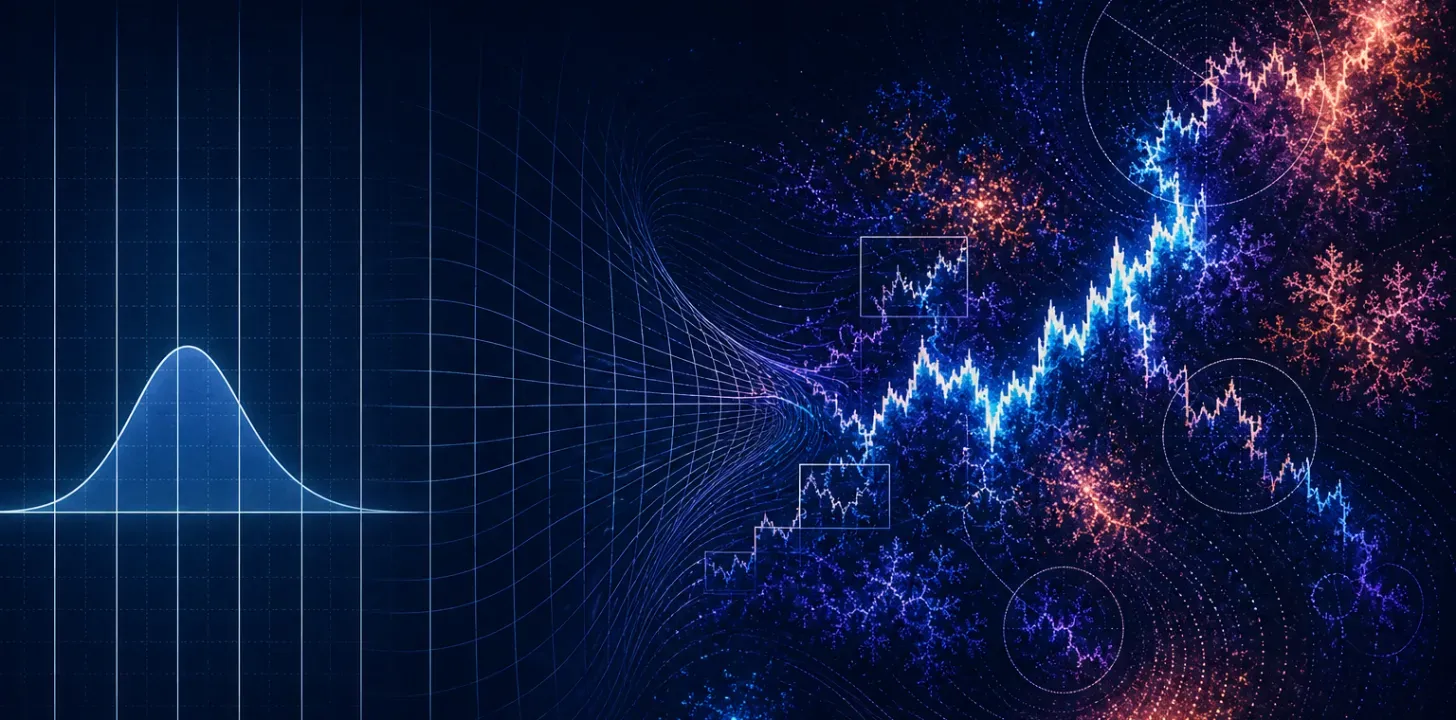
A circle has a radius. A straight line has a direction. These ideal shapes let us describe complicated things with very little information. Their usefulness comes from what they leave out.
A coastline presents a different problem. Look more closely and new bays, inlets, and rocks appear. A shorter ruler follows details that a longer ruler skips, changing the measured length. Over a range of scales, irregularity remains part of the object rather than disappearing with closer inspection. This was one of Mandelbrot’s starting points for a geometry of roughness [1]Mandelbrot, B. “How Long Is the Coast of Britain? Statistical Self-Similarity and Fractional Dimension.” Science, vol. 156, no. 3775, 1967, pp. 636–638..
Financial markets raise a related question: which details can a model safely leave out? A market can drift quietly for weeks and then compress a year’s worth of anxiety into one afternoon. If a model smooths away that concentration of activity, it may simplify away precisely the behavior we need to understand.
Fractal models begin by asking whether those irregularities have a statistical structure of their own.
Ideal shapes and rough reality
Fractal geometry offers a way to describe roughness that persists as we change scale. In an exact mathematical fractal, structure can repeat indefinitely. In a coastline, resemblance is statistical and limited to a range of scales. A small bay is not a scale model of a large one.
The distinction matters for markets, too. A fractal price model does not require a recognizable chart pattern to repeat every hour, day, and month. It concerns how the statistics of price changes behave across those horizons.
There is also a subtlety in the comparison with conventional finance: Brownian motion is already rough and statistically self-similar. Its paths are not smooth Euclidean curves. The limitation of the simplest financial benchmark is more specific: it assumes a uniform statistical rhythm. Multifractal models let that rhythm vary across time and scale.
What the Gaussian benchmark captures—and misses
A standard starting point for financial prices is geometric Brownian motion, or GBM. Imagine rolling similar dice at regular intervals. One roll does not affect the next, and each roll comes from the same distribution. Price changes compound, keeping the price positive.
In GBM, log returns over equal intervals are independent and Gaussian, with constant volatility. This framework helped make option pricing mathematically manageable; it underlies the classic Black–Scholes model [1]Black, F. and M. Scholes. “The Pricing of Options and Corporate Liabilities.” Journal of Political Economy, vol. 81, no. 3, 1973, pp. 637–654..
Real markets repeatedly depart from that benchmark in three ways:
- Extreme moves occur more often than a fitted Gaussian distribution suggests. These heavier tails matter when estimating plausible losses.
- Large moves cluster together. Their direction may change, but their size remains elevated. Quiet periods also tend to persist.
- Behavior changes with the observation horizon. The distribution of minute-by-minute returns does not rescale cleanly into the distribution of monthly returns.
These are recurring empirical patterns, often called financial “stylized facts” [1]Cont, R. “Empirical Properties of Asset Returns: Stylized Facts and Statistical Issues.” Quantitative Finance, vol. 1, no. 2, 2001, pp. 223–236..
Financial modeling already has ways to address some of them. ARCH and GARCH models, for example, allow volatility to change with past conditions [1]Engle, R. F. “Risk and Volatility: Econometric Models and Financial Practice.” Nobel Prize Lecture, 2003..
The particular appeal of multifractal models is that they connect the uneven distribution of activity with behavior across time scales. To see why that connection is useful, consider turbulent water.
Turbulence: bursts within bursts
Watch water rushing past a bridge pillar. Large swirls form, smaller swirls appear within the flow, and agitation varies sharply from place to place. In ordinary three-dimensional turbulence, energy transfers from larger motions toward smaller scales, where viscosity ultimately dissipates it.
That transfer is uneven. Intense fluctuations concentrate in patches and bursts. Physicists call this intermittency. An average describes the overall activity, but conceals how unevenly that activity is distributed. Understanding turbulence therefore requires studying both scale and the concentration of extremes [1]Cleve, J., M. Greiner, B. R. Pearson, and K. R. Sreenivasan. “On the Intermittency Exponent of the Turbulent Energy Cascade.” 2004..
Markets offer a statistical parallel. Quiet intervals alternate with bursts of large price changes. Within an unsettled week, a few hours may carry much of the movement; within those hours, a few minutes may dominate.
This analogy has a research history. In 1996, Ghashghaie and colleagues compared foreign-exchange fluctuations with hydrodynamic turbulence and proposed a corresponding information cascade [1]Ghashghaie, S., W. Breymann, J. Peinke, P. Talkner, and Y. Dodge. “Turbulent Cascades in Foreign Exchange Markets.” Nature, vol. 381, 1996, pp. 767–770..
The proposed connection was challenged almost immediately. Similar statistics do not establish identical mechanisms: a financial market has no established counterpart to the physical energy cascade that would make the two systems interchangeable [1]Arneodo, A., J.-P. Bouchaud, R. Cont, J.-F. Muzy, M. Potters, and D. Sornette. “Comment on ‘Turbulent Cascades in Foreign Exchange Markets.’” 1996..
The useful connection is mathematical. A multiplicative cascade distributes activity unevenly across successive scales. Divide a time interval into pieces and give some pieces more activity than others. Divide again and repeat. A relatively active interval can contain an even more active subinterval, producing bursts nested within bursts.
This is where the vocabulary divides. A monofractal process has one scaling exponent governing its statistical rescaling. A multifractal process allows richer scaling: small fluctuations and large bursts need not change with the observation horizon in the same way.
This gives roughness an internal organization. It also suggests a way to model market time.
Two clocks for the same market
Calendar time advances uniformly: one minute per minute. A modeled trading clock can advance at different speeds. During a quiet interval it moves slowly; during intense activity it races forward. It represents accumulated activity rather than a literal count of trades.
The Multifractal Model of Asset Returns, or MMAR, combines a random price process with a multifractal trading clock. In its Brownian version, more trading time passing during a calendar interval means greater variance of the return over that interval. The clock changes the size of the opportunities for movement without choosing their direction.
This construction can generate heavy tails, persistent dependence in the size of returns, and different scaling behavior for different statistical moments—typical moves and extreme moves can rescale differently as the horizon changes—while keeping raw returns uncorrelated [1]Mandelbrot, B., A. Fisher, and L. Calvet. “A Multifractal Model of Asset Returns.” Cowles Foundation Discussion Paper no. 1164, 1997..
Imagine two ten-minute intervals. In one, prices barely move. In the other, consequential changes arrive in rapid succession. The wall clock gives both intervals the same weight. The activity clock gives the second much more weight.
Activity per interval (% of total)
Elapsed time (% of period)
Activity per interval (% of total)
Elapsed time (% of period)
Cumulative activity (% of total)
Elapsed time (% of period)
Does market direction have memory?
A market can remember the size of recent movements without remembering their direction. A volatile afternoon may be followed by another volatile afternoon, while prices remain capable of either rising or falling.
The activity clock describes this uneven intensity. A separate parameter, the Hurst exponent H, lets us explore dependence in the underlying fluctuations:
- H = ½: Brownian increments are independent.
- H > ½: fractional Brownian increments are positively correlated. Movements tend to reinforce one another.
- H < ½: fractional Brownian increments are negatively correlated. Movements tend to offset one another.
These are statistical tendencies, not instructions for the next move. H is not a correlation coefficient: H = 0.6 does not mean a 60% chance that the next return continues the previous one. An uneven clock also changes the observed calendar-time dependence.
There are empirical reasons to explore persistence. Di Matteo and colleagues found differences in generalized Hurst estimates across developed and emerging markets, with emerging markets tending toward higher estimates [1]Di Matteo, T., T. Aste, and M. M. Dacorogna. “Long-term Memories of Developed and Emerging Markets: Using the Scaling Analysis to Characterize Their Stage of Development.” Journal of Banking & Finance, vol. 29, 2005, pp. 827–851..
However, H above ½ is not an established universal property of markets. The result depends on the instrument, period, horizon, and estimation method. Lo found that evidence of long-range dependence disappeared in the stock-index samples he studied after accounting for short-term dependence [1]Lo, A. W. “Long-term Memory in Stock Market Prices.” NBER Working Paper no. 2984, 1989; published in Econometrica, 1991..
The measured series matters too. Estimates from returns, absolute returns, and volatility describe different properties. In a multifractal analysis, generalized exponents H(q) also depend on the moment being measured, where the index q sets how much weight extreme moves receive. Fat tails can affect measured multiscaling even when returns have been shuffled to remove temporal dependence [1]Barunik, J., T. Aste, T. Di Matteo, and R. Liu. “Understanding the Source of Multifractality in Financial Markets.” 2012..
So the honest answer is conditional. Some series, in some periods, at some horizons, show dependence in direction; none of it generalizes into a property of markets as such.
Aftershocks and the difference between risk and prediction
Earthquakes provide another useful comparison. After a large earthquake, aftershocks become more likely, and their rate generally declines with time. Seismologists estimate the changing likelihood of further events without specifying the exact time and size of the next one [1]U.S. Geological Survey. “Aftershock Forecast Overview.”.
This helps clarify a distinction in finance: knowing that conditions favor large movements is different from knowing which movement comes next. Volatility can remain elevated while the direction of the next return remains difficult to forecast.
The comparison illustrates conditional risk. It does not imply that markets obey earthquake laws or that volatility clustering proves a market is multifractal.
Together, these scientific examples separate three ideas that are easy to blur: coastlines make scale visible, turbulence illustrates concentrated activity across scales, and aftershocks show how risk can change without making individual events predictable.
Try the idea in the market turbulence experiment
My market turbulence experiment makes the activity clock visible. The sticky controls let you explore H separately from activity concentration and pin a result for comparison.
It starts at H = ½ and offers H = 0.6 as a persistent scenario, rather than as a calibrated setting for a typical market. The selected H specifies the model; an estimated H from one simulated path is a noisy diagnostic that rarely matches it exactly. Allowing H to differ from ½ makes this a generalized fractional-Brownian-clock experiment, and it changes the financial assumptions: the Brownian model’s usual martingale and pricing arguments do not automatically carry over.
- Start with uniform activity. Move Activity concentration all the way left. The two price paths coincide: they use the same random shocks and a uniform clock.
- Concentrate the activity. Raise the slider. Read down the page: activity accumulates unevenly, the clock steepens, and larger return fluctuations concentrate in particular intervals. Both models retain the same end-of-year log-price variance; their realized volatility can differ.
- Explore dependence separately. In the sticky controls, with concentration at zero, try Persistent · 0.6 and Reversal · 0.3. Then reintroduce concentration. With no result pinned, both paths use the selected H, so their difference isolates the clock. The uniform-clock reference is GBM only at H = ½. Use Pin this result to preserve a path, then change λ or H to compare settings with the same seed; Clear pin restores the uniform-clock reference.
- Repeat the experiment. Select New realization, then Compare 100 realizations. The comparison reports typical results and their spread across samples. At H = ½, look for persistence in return size without systematic correlation in return direction. Above or below ½, compare how raw-return correlation changes across realizations.
- Explore the geometry separately. Open How fractals repeat across scales and increase recursion depth. Compare regular and scrambled constructions. The cartoon explains repeated geometry; it is a separate illustration from the stochastic clock experiment.
Open Inspect the statistics for return histograms, raw- and absolute-return autocorrelation, Hurst estimates, and estimated singularity spectra. Those estimates are noisy: a finite Gaussian sample will rarely report exactly zero excess kurtosis or a spectrum width of zero. You can also download the paired data or copy a reproducible experiment link.
What changes about our understanding of risk?
Risk is also a question of survival: can you absorb losses as they arrive? Average volatility does not tell you whether a bad year unfolds gradually or whether much of its damage arrives before you can respond.
A thousand small shocks spread over time can leave room to earn income, rebuild reserves, or reduce exposure. A concentrated loss can exhaust those reserves immediately. Small losses are not harmless, and percentage losses do not simply add up—repeated drawdowns can cause ruin on their own. The crucial difference is whether damage arrives faster than the capacity to absorb it can recover.
Consider a simplified balance sheet: €100 of assets financed with €90 of debt and €10 of equity. An immediate 10% fall in asset value wipes out the equity: the debt does not shrink with the assets. Demands for more collateral can force a sale even before that point. A later price recovery is little comfort to someone whose position has already been liquidated. The path to an outcome matters because you may not survive to reach it.
Nassim Nicholas Taleb and Raphael Douady connect fragility to nonlinear responses and sensitivity to increased variability, explicitly including exposure to model error [1]Taleb, N. N. and R. Douady. “Mathematical Definition, Mapping, and Detection of (Anti)Fragility.” Preprint, 2012..
A related idea, asymmetric exposure, concerns the shape of the payoff itself: the frequency of gains says little about the size of the losses that remain possible. A strategy can collect small profits repeatedly while carrying an occasional loss large enough to erase years of gains or end the strategy altogether. A high proportion of profitable days is therefore not, by itself, evidence of safety.
Asymmetry and fragility are related but distinct: gains and losses can be unequal, while fragility concerns how outcomes deteriorate as variability increases. In a leveraged position, a larger shock can cross a collateral or solvency threshold and force liquidation. The resulting damage can grow disproportionately to the initial price movement.
This also challenges confidence in any improved model, including a multifractal one. We need to ask what happens when its estimates are wrong. How much can be gained when conditions are favorable, how much can be lost when they deteriorate, and can the position survive a worse outcome than the model suggests?
Concentration and dependence make different contributions to this problem. Concentrated activity creates short windows of large fluctuations, in either direction. Positive dependence in signed returns can produce sustained runs, including runs of losses. There is also a separate form of dependence: different assets or institutions suffering losses together. A portfolio can contain many holdings yet offer little protection if they share the same vulnerability. This cross-asset dependence is distinct from H and is not modeled by the single-asset experiment here.
The 2008 financial crisis gives this distinction practical weight. The Senior Supervisors Group found that vulnerable firms combined high leverage with excessive reliance on continued secured funding. Those firms underestimated the liquidity risk of concentrated positions and the possibility that financing would become unavailable under stress. The group’s review also identified weaknesses in stress tests, including insufficient attention to market-wide stress occurring alongside trouble at an individual firm [1]Senior Supervisors Group. “Risk Management Lessons from the Global Banking Crisis of 2008.” October 21, 2009..
This can trigger a liquidation spiral: falling asset values lead lenders to demand more collateral, borrowers are forced to sell assets to raise cash, and those sales push prices lower, triggering further forced selling. Then–New York Fed president Timothy Geithner described this self-reinforcing margin spiral in June 2008 [1]Geithner, T. F. “Reducing Systemic Risk in a Dynamic Financial System.” Federal Reserve Bank of New York, June 9, 2008.. The resulting damage can extend beyond the initial losses as financing becomes harder to obtain.
That history supports a criticism of risk models and their use: assumptions about available funding and manageable exposures were too reassuring. It does not establish that a fractal model would have predicted or prevented the crisis. A richer description of price fluctuations still needs to be connected to leverage, collateral requirements, liquidity, and the behavior of other market participants.
The practical questions become more demanding:
- How much can be lost before there is time to act? Examine severe drawdowns and clustered losses, alongside average volatility. Scaling daily risk by the square root of time assumes independent, constant-variance increments; those assumptions need checking.
- What happens when protection weakens at the same time? Stress-test simultaneous losses, reduced diversification, higher collateral demands, and the loss of funding.
- Where is the point of failure? Identify the scenarios that exhaust cash or capital, and assess whether reserves and exposure limits leave enough room to survive them.
Multifractal models help make uneven activity and behavior across time scales explicit. Whether they improve a particular risk estimate requires calibration, comparison with alternatives, and testing on unseen data. Their practical contribution is to sharpen the question: can a position withstand the concentration and sequence of losses, including the actions those losses force? A model that describes the average well can still leave that question unanswered.
For the balance-sheet and funding context, see the Global Liquidity Monitor and Understanding debt service ratios.
Where the research goes next
The next challenge is to connect the statistical shape of market fluctuations with the mechanisms that produce them and the decisions they inform. Recent research points toward models that describe several assets, operate across time scales, and connect volatility to trading activity. The following working papers and preprints, available as of September 2026, illustrate developing directions rather than a settled replacement for existing methods.
Bringing roughness and multifractality into one framework. Zarhali, Bacry, and Muzy develop a model connecting rough and multifractal volatility across multiple assets, with an application to S&P 500 market data. The ambition is to describe both individual volatility and its dependence across assets within a common construction [1]Zarhali, O., E. Bacry, and J.-F. Muzy. “From Rough to Multifractal Multidimensional Volatility: A Multidimensional Log S-fBM Model.” Preprint, revised June 25, 2026.. Here, H describes the roughness of log-volatility; it is not the H controlling dependence in underlying return increments in this article’s experiment.
Asking when diversification actually protects us. Dependence between assets can vary with the observation horizon and the size of the movements being studied. Kakinaka and Umeno propose using multifractal cross-correlation analysis to construct portfolios that account for those differences. They report lower drawdown and tail-risk measures than a mean–variance benchmark in their experiments [1]Kakinaka, S. and K. Umeno. “Portfolio Allocation under Heterogeneous Scales and Multifractality.” Preprint, August 5, 2026.. The practical question is whether assets continue to protect one another during the fluctuations that cause the most damage. The reported advantages await independent replication.
Deriving bursts from trading mechanisms. In related rough-volatility research, Horst, Xu, and Zhang build a model from market orders, limit orders, and cancellations whose arrivals stimulate further activity. Their mathematical construction produces volatility spikes and clusters of spikes [1]Horst, U., W. Xu, and R. Zhang. “Path-dependent Fractional Volterra Equations and the Microstructure of Rough Volatility Models Driven by Poisson Random Measures.” Preprint, December 21, 2024.. This offers a route from a statistical description toward an explanation of how trading can generate irregularity.
Checking which patterns survive measurement. A study of Bitcoin realized volatility by Pontiggia examines how roughness estimates change with sampling frequency, observation window, and the way volatility is measured. The estimates vary with those choices, and the findings concern observed realized volatility rather than directly identifying the roughness of the underlying, unobserved volatility process [1]Pontiggia, M. “Pathwise Roughness of Bitcoin Realized Volatility: Stability Across Time, Sampling, and Volatility Measures.” Preprint, revised July 23, 2026.. Establishing which patterns are robust is essential before treating them as general properties of markets.
For economic modeling, the opportunity is to connect these descriptions of fluctuations with balance sheets, funding constraints, and institutional behavior. A compact statistical model could then inform questions about how shocks spread and when losses become impossible to absorb. These papers explore parts of that connection.
The ambition is an economy of explanation: a small set of principles that accounts for several observed patterns across markets and horizons. Success will require those principles to produce stable estimates, useful forecasts on unseen data, and better assessments of what a portfolio or institution can survive.
What a better model still cannot tell us
A multifractal model does not identify what will trigger the next crisis. Its parameters depend on the data, observation frequency, and estimation method. Apparent scaling over one range of horizons need not continue outside it or survive a change in market conditions.
These limits belong alongside the model’s strengths. Reproducing historical patterns can improve the questions we ask about risk, but it does not guarantee better forecasts or turn a simulated path into a trading signal.
A useful market model must account for both the quiet afternoon and the violent week. Fractal models make the uneven distribution of activity part of the description. Their value lies in helping us ask how risk accumulates across time—and how much an average can conceal.